

Consuming Japan

Winners' Circles (Analyzing Networks with Pajek)
Categories:
There is more to social network analysis than visualizing networks. This section provides a brief overview of the analytic tools that Pajek provides and how to read the tables these tools generate.
In the previous section, we saw how adding visual information to network diagrams highlights structures and points to questions of interest. But as all network analysts know, adding too much information can make a network incomprehensible. Figure 7 is a case in point.
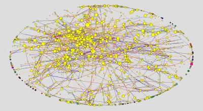
Here the network in question is from 2006, a year in which 2,662 creators participated in creating 808 winning ads. The colors distinguish Ads (Yellow) from Creators (Green). The sizes of the nodes indicate the number of edges connecting each node to its immediate neighbors. The colors of the lines indicate the roles that connect individual creators to the ads on which they worked. The result is unintelligible to the human eye.
The inability of the human eye to parse large and richly coded networks means that, for practical purposes, most empirical network analysis becomes either computational, using software to crunch numbers and pondering the results, or requires dissection of large networks into subnetworks. In practice, these two approaches are frequently combined, and Pajek provides numerous tools for these purposes. Using Pajek, we can
find clusters (components, neighbourhoods of ?eimportant’ vertices, cores, etc.) in a network, extract vertices that belong to the same clusters and show them separately, possibly with the parts of the context (detailed local view), shrink vertices in clusters and show relations among clusters (global view).(Bataglej, 2008:8)
At the same time, we can use the Info command to examine the numbers generated by Pajek during these and other operations. Continuing, then, with Ads-Creators 2006, the network illustrated in Figure 7, we begin with Info>Network>General. In the Info report window we see the following table.
Number of vertices (n): 3469
——————————————————————————-
Arcs Edges
——————————————————————————-
Number of lines with value=1 0 1079
Number of lines with value#1 0 6195
——————————————————————————-
Total number of lines 0 7274
——————————————————————————-
Number of loops 0 0
Number of multiple lines 0 1102
——————————————————————————-
Density1 [loops allowed] = 0.0012089
Density2 [no loops allowed] = 0.0012093
Average Degree = 4.1937158
2-Mode Network: Rows=808, Cols=2661
Density [2-Mode] = 0.0033831
Reading from the top, we see that the network contains a total of 3469 nodes (here called vertices). If this were a directed network, we would have to distinguish between Arcs and Edges. In this network, however, there are no Arcs. All of the lines are undirected Edges and represent relations in which the relationship between node A and node B is the same as that between node B and node A.
In the next block we see that the number of lines with value equal to 1 is 1079, while the number of lines with value not equal to 1 is 6195. Here, however, we have to be careful. The ways in which Pajek presents numbers like these are very general and highly abstract. Pajek only reports the results of calculations without differentiating what these numbers might mean. In some cases, the numbers of lines equal or not equal to one are structural properties resulting from calculations. Here, however, the numbers are assigned codes that indicate the roles that connect Creators to Ads (1=Copywriter, 2=Creative Director, 3=Art Director, 4=Designer, 5=Photographer, 6=Planner, 7=Producer, 8=Film Director, 9=Cameraman, and 99=Other). The numbers are, in other words, only labels in classification; they correspond to the line colors that appear in the network diagram and can be used to select particular sets of lines. They should not, however, be used in calculations.
The next two blocks tell us that the total number of lines is 7,274, of which 1,102 are multiple lines. These numbers are significant, since they tell us that some pairs of nodes are connected more than once (in this case because the same creator may play multiple roles in the team that produces an ad) and allow us to calculate that, in this case, 15.1% of creators have played multiple roles. The number of loops, edges that connect a node to itself, is 0. This is an artifact of our data, a 2-mode (bipartite) network in which which a node of one type can only be connected to a second node of the other type (Ads to Creators or vice-versa).
The next set of numbers provide us with two common measures of network structure: Density and Degree. Density is the percentage of edges found in the data when compared to the total number of possible edges (n(n-1)/2) in a network with n nodes). As a result, Density tends to decline as network size increases. Degree, the number of neighboring nodes directly connected to the the node in question, is a more informative measure. The 4.1937158 reported here could, however, be misleading. It tells us that, on average, every node in this 2-mode network is connected on average to between 4 and 5 nodes of the opposite type. It does not tell us either the average number of creators involved in producing an ad or the average number of ads produced by a single creator. To discover these facts requires further analysis.
The last set of numbers tells us that, if this 2-mode network were represented by a matrix, the matrix would have 808 rows and 2661 columns. For mathematical purposes, networks are often represented as matrixes and methods from matrix algebra are used to analyze them. Here the rows are Ads, the columns Creators, and a non-zero number in a cell where a row and a column intersect indicates that there is a relationship between the Ad and Creator in question. In this case, the commands Net>Partition>2-mode and Info>Partition produce the following table.
Dimension: 3469
The lowest value: 1
The highest value: 2
Frequency distribution of cluster values:
Cluster Freq Freq% CumFreq CumFreq% Representative
———————————————————————————————-
1 808 23.2920 808 23.2920 AD1_06
2 2661 76.7080 3469 100.0000 Yam342
———————————————————————————————-
Sum 3469 100.0000
Here we find little that we do not already know. The table tells us that we are looking at partition that divides the total network into two clusters labeled 1 and 2 of which the first contains 808 members, the second 2661. Since these are the Ads and Creators, there is nothing new for us here. Digging a bit deeper, we find that yellow and green are the default colors that Pajek assigns to clusters numbered 1 and 2. We also note the column headers: Freq=frequency; Freq%=percentage of total; CumFreq=Cumulative Frequency; CumFreq%=cumulative percentage of total; and Representative is simply an identifier for a typical example of the cluster. With only two clusters to worry about, this may seem a lot of bother for no great reward. Suppose, however, that we change the partition by using Net>Partition>Degree>All and Info>Partition. Now the table that appears is the following
Dimension: 3469
The lowest value: 1
The highest value: 60
Frequency distribution of cluster values:
Cluster Freq Freq% CumFreq CumFreq% Representative
———————————————————————————————-
1 1261 36.3505 1261 36.3505 Tan1892
2 623 17.9591 1884 54.3096 AD760_06
3 255 7.3508 2139 61.6604 AD83_06
4 277 7.9850 2416 69.6454 AD103_06
5 229 6.6013 2645 76.2468 AD5_06
6 183 5.2753 2828 81.5221 AD67_06
7 99 2.8538 2927 84.3759 AD38_06
8 104 2.9980 3031 87.3739 AD76_06
9 76 2.1908 3107 89.5647 AD60_06
10 54 1.5566 3161 91.1214 AD43_06
11 39 1.1242 3200 92.2456 AD104_06
12 50 1.4413 3250 93.6869 AD1_06
13 32 0.9225 3282 94.6094 AD22_06
14 21 0.6054 3303 95.2148 AD65_06
15 27 0.7783 3330 95.9931 AD15_06
16 16 0.4612 3346 96.4543 AD13_06
17 25 0.7207 3371 97.1750 AD80_06
18 16 0.4612 3387 97.6362 AD19_06
19 12 0.3459 3399 97.9821 AD37_06
20 17 0.4901 3416 98.4722 AD73_06
21 7 0.2018 3423 98.6740 AD75_06
22 3 0.0865 3426 98.7604 AD450_06
23 5 0.1441 3431 98.9046 AD366_06
24 6 0.1730 3437 99.0775 AD195_06
25 6 0.1730 3443 99.2505 AD210_06
26 3 0.0865 3446 99.3370 Ich674
27 1 0.0288 3447 99.3658 Sas1520
28 4 0.1153 3451 99.4811 AD448_06
29 1 0.0288 3452 99.5099 Ter536
31 6 0.1730 3458 99.6829 AD315_06
32 1 0.0288 3459 99.7117 Yam342
34 5 0.1441 3464 99.8559 AD311_06
39 1 0.0288 3465 99.8847 Soe903
42 1 0.0288 3466 99.9135 Oka258
49 2 0.0577 3468 99.9712 Sas3
60 1 0.0288 3469 100.0000 Saw8
———————————————————————————————-
Sum 3469 100.0000
Here we learn that Degree, the number of immediate neighbors of nodes, ranges from 1 to 60. We may also note that the Representative nodes for the top four numbers are all Creators instead of Ads. We may also note the highly skewed distribution of degrees, from 1,261 nodes with only one immediate neighbor to only 1 node with 60 immediate neighbors. What could these observations means?
The commands that generated the Degree partition also created a Degree vector. We have already noted that the cluster numbers in partitions are only labels for discrete categories. These can be handy for extracting subnetworks of nodes belonging to those categories but cannot, being only labels, be used in calculations. The numbers in vectors are real numbers (pun intended). They can be used in calculations. If we have already used Net>Partition>Degree>All as indicated above, Info>Vector produces the following table
Dimension: 3469
The lowest value: 0.0003
The highest value: 0.0173
——————————————————————-
Sum (all values): 4.1949
Arithmetic mean: 0.0012
Median: 0.0006
Standard deviation: 0.0014
2.5% Quantile: 0.0003
5.0% Quantile: 0.0003
95.0% Quantile: 0.0040
97.5% Quantile: 0.0052
Vector Values Frequency Freq% CumFreq CumFreq%
——————————————————————————————————————————
( ... 0.000] 1261 36.3505 1261 36.3505
( 0.000 ... 0.006] 2155 62.1216 3416 98.4722
( 0.006 ... 0.012] 49 1.4125 3465 99.8847
( 0.012 ... 0.017] 4 0.1153 3469 100.0000
——————————————————————————————————————————
Total 3469 100.0000
Here we find the kinds of numbers used in statistical analysis: the range, mean, median, standard deviation, and the points one, two, three and four standard deviations from the mean. In the table the label of on the label on the leftmost column has changed from “Cluster” to “Vector Values,” and the numbers in the leftmost column have changed from integers used as labels to ranges defined in terms of real numbers.
In this section, we have learned that Pajek can be used to dissect as well as analyze whole networks and begun to get a sense of how to think about the numbers that Pajek generates the diagrams with which we begin our explorations of our primary data: the 2-mode networks in which the members of winning teams and the ads they created are nodes and the roles that linked creators to ads the ties that connect them.
Next entry: Dogû, a Cosmos
Previous entry: Winners' Circles (Visualizing Networks with Pajek)